Bayesian replication test
In a very cool paper on different types of replication tests, Verhagen and Wagenmakers proposed their own variant of a Bayesian replication test (see reference below). The test compares the “proponent’s” hypothesis that the new data constitute a replication against the “skeptic’s” hypothesis that the new data constitutes a null effect. The presents simulations comparing the different Bayesian and frequentist measures, and makes a compelling argument for the proposed new measure.
For the case of a t-test, Verhagen and Wagenmakers show how one can approximate the evidential support (Bayes Factor) for the replication hypothesis over the null hypothesis, BF_r0, based on just
- the t-statistics of the original and new data
- the number of data points in the original t-test and t-test over the replication data
It occurred to me that one might be able to use the same measure to assess the replicability of individual effects in linear mixed models (i.e., the evidentiary support for the hypothesis that a specific effect in a multiple linear regression model replicates), in particular in cases where the different predictors in the model are all orthogonal to each other (e.g., in balanced designs). So one purpose of this post is to give everyone something to shout at if they disagree.
The second purpose is to post the code here. The code is really all from Josine Verhagen’s webpage. I’m posting it here for convenience. But I just
- wrote a quick and dirty wrapper function that uses the lmerTest and pbkrtest packages to provide Satterthwaite (fast and often good for large data sets) or Kenward-Roger (more precise, but a lot slower and ever more so, the larger the data) approximations of the degrees of freedom for the t-test, which are used to get the ‘number of data points’ that went into the original and replication t-test.
- update the plotting of the prior and posterior densities to use ggplot2, so that the plot can be more easily modified subsequently.
For documentation and background, please see Verhagen and Wagenmaker’s excellent paper!
whichDFMethod <- function(model) {
  l = length(fitted(model))

  # This threshold was set more or less arbitrarily, based on some
  # initial testing. You might want to change it. Satterthwaite's
  # approximation can result in hugely inflated DFs.
  if (l < 3000) {
    cat(paste0("Using Kenward-Roger's approximation of DFs for t-test over coefficient because the data set is small: ", l, "\n"))
    return("Kenward-Roger")
  } else { return("Satterthwaite") }
}

# wrapper function that calls ReplicationBayesfactorNCT with t-values and n1, n2 observations
# based on the output of mixed model analyses. The test is conducted for the k=th t-test within
# the mixed model, specified by the "coef" argument. Assumes that the models have been fit with lmerTest,
# so that the approximated DFs can be used as n1 and n2 (number of observations in the original and
# replication experiment). For that reason (and only that reason), the function requires lmerTest.
replicationBF <- function(model1, model2, yhigh = 0, limits.x = NULL, coef = 1, M = 500000) {
  require(lmerTest)
  require(pbkrtest)

  summary1 = summary(model1, ddf=whichDFMethod(model1))
  summary2 = summary(model2, ddf=whichDFMethod(model2))

  print(summary1)
  cat("\n\n")
  print(summary2)

  cat("\n\nCalculting replication Bayes Factor:\n")
  out <- ReplicationBayesfactorNCT(
    coef(summary1)[coef,"t value"],
    coef(summary2)[coef,"t value"],
    coef(summary1)[coef,"df"] + 1, # Since the ReplicationBayesfactorNCT function subtracts 1 for the DFs (for sample == 1)
    coef(summary2)[coef,"df"] + 1, # Since the ReplicationBayesfactorNCT function subtracts 1 for the DFs (for sample == 1)
    sample = 1,
    plot = 1,
    post = 1,
    yhigh = yhigh,
    limits.x = limits.x,
    M = M
  )

  return (out)
}

# Replication Bayes Factor taken from Josine Verhagen's webpage
# (http://josineverhagen.com/?page_id=76).
# See Verhagen and Wagenmakers (2014) for details.
#
# Minor modifications to the plotting made by fjaeger@ur.rochester.edu
ReplicationBayesfactorNCT <- function(
  tobs,                  # t value in first experiment
  trep,                  # t value in replicated experiment
  n1,                    # first experiment: n in group 1 or total n
  n2,                    # second experiment: n in group 1 or total n
  m1       = 1,          # first experiment: n in group 2 or total n
  m2       = 1,          # second experiment: n in group 2 or total n
  sample   = 1,        # 1 = one sample t-test (or within), 2 = two sample t-test
  wod      = dir,	      # working directory
  plot = 0,  # 0 = no plot 1 = replication
  post = 0,  # 0 = no posterior, 1 = estimate posterior
  M = 500000,
  yhigh = 0,
  limits.x = NULL
)
{
  require(MCMCpack)
  require(ggplot2) # added by TFJ

  ##################################################################
  #STEP 1: compute the prior for delta based on the first experiment
  ################################### ###############################

  D    <- tobs

  if (sample==1) {
    sqrt.n.orig  <-  sqrt(n1)
    df.orig <- n1 -1
  }

  if (sample==2) {
    sqrt.n.orig  <- sqrt( 1/(1/n1+1/m1)) # two sample alternative for sqrt(n)
    df.orig <- n1 + m1 -2   #degrees of freedom
  }

  # To find out quickly the lower and upper bound areas, the .025 and .975 quantiles of tobs at a range of values for D are computed.
  # To make the algorithm faster, only values in a reasonable area around D are computed.
  # Determination of area, larger with large D and small N
  range.D <- 4 + abs(D/(2*sqrt.n.orig))
  sequence.D <- seq(D,D + range.D,.01) #make sequence with range
  # determine which D gives a quantile closest to tobs with an accuracy of .01
  options(warn=-1)
  approximatelow.D <- sequence.D[which( abs(qt(.025,df.orig,sequence.D)-tobs)==min(abs(qt(.025,df.orig,sequence.D)-tobs)) )]
  options(warn=0)
  # Then a more accurate interval is computed within this area
  # Make sequence within .01 from value found before
  sequenceappr.D <- seq((approximatelow.D-.01),(approximatelow.D+.01),.00001)
  # determine which D gives a quantile closest to tobs with an accuracy of .00001
  low.D <- sequenceappr.D[which( abs(qt(.025,df.orig,sequenceappr.D)-tobs)==min(abs(qt(.025,df.orig,sequenceappr.D)-tobs)) )]

  # Compute standard deviation for the corresponding normal distribution.
  sdlow.D <- (D-low.D)/qnorm(.025)

  # compute prior mean and as for delta
  prior.mudelta <- D/sqrt.n.orig
  prior.sdelta <-  sdlow.D/sqrt.n.orig

  ##################################################################
  #STEP 2: Compute Replication Bayes Factor
  ##################################################################
  # For one sample t-test: within (group2==1) or between (group2==vector)

  if (sample==1)
  {
    df.rep <- n2-1
    sqrt.n.rep <- sqrt(n2)
    Likelihood.Y.H0 <- dt(trep,df.rep)

    sample.prior <- rnorm(M,prior.mudelta,prior.sdelta)
    options(warn=-1)
    average.Likelihood.H1.delta <- mean(dt(trep,df.rep,sample.prior*sqrt.n.rep))
    options(warn=0)

    BF <- average.Likelihood.H1.delta/Likelihood.Y.H0
  }

  # For two sample t-test:

  if (sample==2)  {
    df.rep <- n2 + m2 -2
    sqrt.n.rep <- sqrt(1/(1/n2+1/m2))
    Likelihood.Y.H0 <- dt(trep,df.rep)

    sample.prior <- rnorm(M,prior.mudelta,prior.sdelta)
    options(warn=-1)
    average.Likelihood.H1.delta <- mean(dt(trep,df.rep,sample.prior*sqrt.n.rep))
    options(warn=0)
    BF <- average.Likelihood.H1.delta/Likelihood.Y.H0
  }

  #################################################################
  #STEP 3: Posterior distribution
  #################################################################


  if( post == 1) {

    options(warn=-1)
    likelihood <- dt(trep,df.rep,sample.prior*sqrt.n.rep)
    prior.density <- dnorm(sample.prior,prior.mudelta,prior.sdelta)
    likelihood.x.prior <- likelihood * prior.density

    LikelihoodXPrior <- function(x) {dnorm(x,prior.mudelta,prior.sdelta) * dt(trep,df.rep,x*sqrt.n.rep) }
    fact  <- integrate(LikelihoodXPrior,-Inf,Inf)
    posterior.density <- likelihood.x.prior/fact$value
    PosteriorDensityFunction <- function(x) {(dnorm(x,prior.mudelta,prior.sdelta) * dt(trep,df.rep,x*sqrt.n.rep))/fact$value }
    options(warn=0)

    mean <- prior.mudelta
    sdh  <- prior.mudelta + .5*(max(sample.prior)[1] - prior.mudelta)
    sdl  <- prior.mudelta - .5*(prior.mudelta - min(sample.prior)[1])
    dev  <- 2

    for ( j in 1:10) {
      rangem <- seq((mean-dev)[1],(mean+dev)[1],dev/10)
      rangesdh <- seq((sdh-dev)[1],(sdh+dev)[1],dev/10)
      rangesdl <- seq((sdl-dev)[1],(sdl+dev)[1],dev/10)
      perc <- matrix(0,length(rangem),3)


      I<-min(length(rangem), length(rangesdh),length(rangesdl) )
      for ( i in 1:I) {
        options(warn=-1)
        vpercm <-  integrate(PosteriorDensityFunction, -Inf,  rangem[i])
        perc[i,1]<- vpercm$value
        vpercsh <-  integrate(PosteriorDensityFunction, -Inf,  rangesdh[i])
        perc[i,2]<- vpercsh$value
        vpercsl <-  integrate(PosteriorDensityFunction, -Inf,  rangesdl[i])
        perc[i,3]<- vpercsl$value
        options(warn=0)
      }
      mean <- rangem[which(abs(perc[,1]-.5)== min(abs(perc[,1]-.5)))]
      sdh <-  rangesdh[which(abs(perc[,2]-pnorm(1))== min(abs(perc[,2]-pnorm(1))))]
      sdl <-  rangesdl[which(abs(perc[,3]-pnorm(-1))== min(abs(perc[,3]-pnorm(-1))))]
      dev <- dev/10
    }

    posterior.mean <- mean
    posterior.sd <- mean(c(abs(sdh- mean),abs(sdl - mean)))
  }

  if (post != 1) {
    posterior.mean <- 0
    posterior.sd <- 0
  }

  ###########OUT

  dat.SD=new.env()
  dat.SD$BF      <- BF
  dat.SD$prior.mean= round(prior.mudelta,2)
  dat.SD$prior.sd= round(prior.sdelta,2)
  dat.SD$post.mean= round(posterior.mean,2)
  dat.SD$post.sd= round(posterior.sd,2)
  dat.SD=as.list(dat.SD)


  ###########################################
  #PLOT
  ###########################################
  if (plot==1)
  {

    if (post != 1) {
      options(warn =-1)
      rp <- ReplicationPosterior(trep,prior.mudelta,prior.sdelta,n2,m2=1,sample=sample)
      options(warn =0)

      posterior.mean <- rp[[1]]
      posterior.sd  <- rp[[2]]
    }

    par(cex.main = 1.5, mar = c(5, 6, 4, 5) + 0.1, mgp = c(3.5, 1, 0), cex.lab = 1.5,
        font.lab = 2, cex.axis = 1.3, bty = "n", las=1)

    high <- dnorm(posterior.mean,posterior.mean,posterior.sd)
    add <- high/5

    if(yhigh==0) {
      yhigh <- high + add
    }

    scale <- 3

    if (is.null(limits.x)) {
      min.x <-  min((posterior.mean - scale*posterior.sd),(prior.mudelta - scale*prior.sdelta))
      max.x <-  max((posterior.mean + scale*posterior.sd),(prior.mudelta + scale*prior.sdelta))
    } else {
      min.x <-  limits.x[1]
      max.x <-  limits.x[2]

    }

    ggplot(
      data = data.frame(x = 0),
      mapping = aes(
        x = x
      )
    ) +
      scale_x_continuous(expression(Effect ~ size ~ delta),
                         limits = c(min.x, max.x)
      ) +
      scale_y_continuous("Density",
                         limits = c(0, yhigh)
      ) +
      stat_function(
        fun = function(x) dnorm(x, prior.mudelta, prior.sdelta),
        aes(linetype = "Before replication"),
        size = .75
      ) +
      stat_function(
        fun = function(x) dnorm(x, posterior.mean, posterior.sd),
        aes(linetype = "After replication"),
        size = 1
      ) +
      scale_linetype_manual("",
        values = c("Before replication" = 2,
                   "After replication" = 1)
      ) +
      geom_point(
        x = 0, y = dnorm(0,prior.mudelta,prior.sdelta),
        color = "gray", size = 3
      ) +
      geom_point(
        x = 0, y = dnorm(0,posterior.mean,posterior.sd),
        color = "gray", size = 3
      ) +
      geom_segment(
        x = 0, xend = 0,
        y = dnorm(0,prior.mudelta,prior.sdelta), yend= dnorm(0,posterior.mean,posterior.sd),
        color = "gray"
      ) +
      annotate(
        geom = "text",
        x = sum(limits.x) / 2, y = yhigh - 1/10 * yhigh,
        label = as.expression(bquote(BF[r0] == .(round(BF, digits=2))))
      ) +
      theme(
        legend.position = "bottom",
        legend.key.width = unit(1.5, "cm")
      )

  }

  return(dat.SD)
}
Verhagen, J., & Wagenmakers, E. J. (2014). Bayesian tests to quantify the result of a replication attempt. Journal of Experimental Psychology: General, 143(4), 1457.
Two post-doc positions available in our lab
- Project 1: Inference and learning during speech perception and adaptation
- Project 2: Web-based self-administered speech therapy
Although we mention preferred specializations below, applicants from any fields in the cognitive and language sciences are welcome. While candidates will join an active project, candidates are welcome/encouraged to also develop their own independent research program. In case of doubt, please contact Florian Jaeger at fjaeger@bcs.rochester.edu, rather than to self-select not to apply.
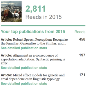
What did you read in 2015?
Another year has passed and academic platform bombard us with end-of-year summaries. So, here are the most-read HLP Lab papers of 2015. Congratulations to Dave Kleinschmidt, who according to ResearchGate leads the 2015 HLP Lab pack with his beautiful paper on the ideal adapter framework for speech perception, adaptation, and generalization. The paper was cited 22 times in the first 6 months of being published! Well deserved, I think … as a completely neutral (and non-ideal) observer ;).
Academia.edu mostly agreed, Read the rest of this entry »
The (in)dependence of pronunciation variation on the time course of lexical planning
Language, Cognition, and Neuroscience just published Esteban Buz’s paper on the relation between the time course of lexical planning and the detail of articulation (as hypothesized by production ease accounts).
Several recent proposals hold that much if not all of explainable pronunciation variation (variation in the realization of a word) can be reduced to effects on the ease of lexical planning. Such production ease accounts have been proposed, for example, for effects of frequency, predictability, givenness, or phonological overlap to recently produced words on the articulation of a word. According to these account, these effects on articulation are mediated through parallel effects on the time course of lexical planning (e.g., recent research by Jennifer Arnold, Jason Kahn, Duane Watson, and others; see references in paper).


This would indeed offer a parsimonious explanation of pronunciation variation. However, the critical test for this claim is a mediation analysis, Read the rest of this entry »
Special issue in “Cross-linguistic Psycholinguistics”
At long last! It’s my great pleasure to announce the publication of the special issue on “Laboratory in the field: advances in cross-linguistic psycholinguistics”, edited by Alice Harris (UMass), Elisabeth Norcliffe (MPI, Nijmegen), and me (Rochester), in Language, Cognition, and Neuroscience. It is an exciting collection of cross-linguistic studies on language production and comprehension and it feels great to see the proofs for the whole shiny issue:

Speech perception and generalization across talkers
We recently submitted a research review on “Speech perception and generalization across talkers and accents“, which provides an overview of the critical concepts and debates in this domain of research. This manuscript is still under review, but we wanted to share the current version. Of couse, feedback is always welcome.
In this paper, we review the mixture of processes that enable robust understanding of speech across talkers despite the lack of invariance. These processes include (i) automatic pre-speech adjustments of the distribution of energy over acoustic frequencies (normalization); (ii) sensitivity to category-relevant acoustic cues that are invariant across talkers (acoustic invariance); (iii) sensitivity to articulatory/gestural cues, which can be perceived directly (audio-visual integration) or recovered from the acoustic signal (articulatory recovery); (iv) implicit statistical learning of talker-specific properties (adaptation, perceptual recalibration); and (v) the use of past experiences (e.g., specific exemplars) and structured knowledge about pronunciation variation (e.g., patterns of variation that exist across talkers with the same accent) to guide speech perception (exemplar-based recognition, generalization).
CUNY 2015 plenary
As requested by some, here are the slides from my 2015 CUNY Sentence Processing Conference plenary last week:
I’m posting them here for discussion purposes only. During the Q&A several interesting points were raised. For example Read the rest of this entry »
HLP Lab at CUNY 2015
We hope to see y’all at CUNY in a few weeks. In the interest of hopefully luring to some of our posters, here’s an overview of the work we’ll be presenting. In particular, we invite our reviewers, who so boldly claimed (but did not provide references for the) triviality of our work ;), to visit our posters and help us mere mortals understand.
- Articulation and hyper-articulation
- Unsupervised and supervised learning during speech perception
- Syntactic priming and implicit learning during sentence comprehension
- Uncovering the biases underlying language production through artificial language learning
Interested in more details? Read on. And, as always, I welcome feedback. (to prevent spam, first time posters are moderated; after that your posts will always directly show)
Some thoughts on Healey et al (2014) failure to find syntactic priming in conversational speech
In a recent PLoS one article, Healey, Purver, and Howes (2014) investigate syntactic priming in conversational speech, both within speakers and across speakers. Healey and colleagues follow Reitter et al (2006) in taking a broad-coverage approach to the corpus-based study of priming. Rather than to focus on one or a few specific structures, Healey and colleagues assess lexical and structural similarity within and across speakers. The paper concludes with the interesting claim that there is no evidence for syntactic priming within speaker and that alignment across speakers is actually less than expected by chance once lexical overlap is controlled for. Given more than 30 years of research on syntactic priming, this is a rather interesting claim. As some folks have Twitter-bugged me (much appreciated!), I wanted to summarize some quick thoughts here. Apologies in advance for the somewhat HLP-lab centric view. If you know of additional studies that seem relevant, please join the discussion and post. Of course, Healey and colleagues are more than welcome to respond and correct me, too.
First, the claim by Healey and colleagues that “previous work has not tested for general syntactic repetition effects in ordinary conversation independently of lexical repetition” (Healey et al 2014, abstract) isn’t quite accurate.
HLP Lab is grinking 2014
And it’s that time of the year again. Time to take stock. This last year has seen an unusual amount of coming and going. It’s been great to have so many interesting folks visit or spend time in the lab.
Grads
- Masha Fedzechkina defended her thesis, investigation what artificial language learning can tell us about the source of (some) language universals. She started her post-doc at UPenn, where she’s working with John Trueswell and Leila Gleitman. See this earlier post.
- Ting Qian successfully defended his thesis on learning in a (subjectively) non-stationary world (primarily advised by Dick Aslin and including some work joint with me). His thesis contained such delicious and ingenious contraptions as the Hibachi Grill Process, a generalization of the Chinese Restaurant Process, based on the insight that the order of stimuli often contains information about the structure of the world so that a rational observer should take this information into account (unlike basically all standard Bayesian models of learning). Check out his site for links to papers under review. Ting’s off to start his post-doc with Joe Austerweil at Brown University.
Post-docs Read the rest of this entry »
Speech recognition: Recognizing the familiar, generalizing to the similar, and adapting to the novel
At long last, we have finished a substantial revision of Dave Kleinschmidt‘s opus “Robust speech perception: Recognize the familiar, generalize to the similar, and adapt to the novel“. It’s still under review, but we’re excited about it and wanted to share what we have right now.

The paper builds on a large body of research in speech perception and adaptation, as well as distributional learning in other domains to develop a normative framework of how we manage to understand each other despite the infamous lack of invariance. At the core of the proposal stands the (old, but often under-appreciated) idea that variability in the speech signal is often structured (i.e., conditioned on other variables in the world) and that an ideal observer should take advantage of that structure. This makes speech perception a problem of inference under uncertainty at multiple different levels Read the rest of this entry »
more on old and new lme4
(This is another guest post by Klinton Bicknell.)
This is an update to my previous blog post, in which I observed that post-version-1.0 versions of the lme4 package yielded worse model fits than old pre-version-1.0 versions for typical psycholinguistic datasets, and I gave instructions for installing the legacy lme4.0 package. As I mentioned there, however, lme4 is under active development, the short version of this update post is to say that it seems that the latest versions of the post-version-1.0 lme4 now yield models that are just as good, and often better than lme4.0! This seems to be due to the use of a new optimizer, better convergence checking, and probably other things too. Thus, installing lme4.0 now seems only useful in special situations involving old code that expects the internals of the models to look a certain way. Life is once again easier thanks to the furious work of the lme4 development team!
[update: Since lme4 1.1-7 binaries are now on CRAN, this paragraph is obsolete.] One minor (short-lived) snag is that the current version of lme4 on CRAN (1.1-6) is overzealous in displaying convergence warnings, and displays them inappropriately in many cases where models have in fact converged properly. This will be fixed in 1.1-7 (more info here). To avoid them for now, the easiest thing to do is probably to install the current development version of lme4 1.1-7 from github like so:
library("devtools"); install_github("lme4/lme4")
Read on if you want to hear more details about my comparisons of the versions.
Congratulations to Dr. Fedzechkina
Congratulations to Masha (a.k.a Dr. Fedzechkina) for successfully defending her thesis “Communicative Efficiency, Language Learning, and Language Universals“, jointly advised by Lissa Newport (now at Georgetown) and me. Masha’s thesis presents 7 multi-day artificial language learning studies that investigate the extent to which functional pressures guide language learning, thereby leading learners to subtly deviate from the input they receive.
Five of the experiments investigate the trade-off between word order and case-marking as a means of encoding grammatical function assignment. For a preview on these experiments, see the short report in Fedzechkina, Jaeger, and Newport (2011) and this paper under review. Two additional experiments investigate how learners trade-off animacy and case-marking (Fedzechkina, Jaeger, & Newport, 2012). Her most recent studies also show how learners trade-off uncertainty (assessed as the conditional entropy over grammatical function assignments given perfect knowledge of the grammar) and effort.

HLP Lab and collaborators at CMCL, ACL, and CogSci
The summer conference season is coming up and HLP Lab, friends, and collaborators will be presenting their work at CMCL (Baltimore, joint with ACL), ACL (Baltimore), CogSci (Quebec City), and IWOLP (Geneva). I wanted to take this opportunity to give an update on some of the projects we’ll have a chance to present at these venues. I’ll start with three semi-randomly selected papers. Read the rest of this entry »
The ‘softer kind’ of tutorial on linear mixed effect regression
I recently was pointed to this nice and very accessible tutorial on linear mixed effects regression and how to run them in R by Bodo Winter (at UC Merced). If you don’t have much or any background in this type of model, I recommend you pair it with a good conceptual introduction to these models like Gelman and Hill 2007 and perhaps some slides from our LSA 2013 tutorial.
There are a few thing I’d like to add to Bodo’s suggestions regarding how to report your results:
- be clear how you coded the variables since this does change the interpretation of the coefficients (the betas that are often reported). E.g. say whether you sum- or treatment-coded your factors, whether you centered or standardized continuous predictors etc. As part of this, also be clear about the direction of the coding. For example, state that you “sum-coded gender as female (1) vs. male (-1)”. Alternatively, report your results in a way that clearly states the directionality (e.g., “Gender=male, beta = XXX”).
- please also report whether collinearity was an issue. E.g., report the highest fixed effect correlations.
Happy reading.
